Michael Crescimanno is a Physics professor at the Youngstown Univer...
Traceroute is a standard utility on most TCP/IP-enabled operating s...
You can see the exact path of your request as well as the number of...
Using the arc length formula $r\theta = s$ for both the Earth and t...
For reverse lookup locations using IP, you can rely on better servi...
Interestingly, when Eratosthenes measured the Earth, the main sourc...
Measuring the Earth with Traceroute
By
Snowflake Kicovic, Loren Webb and Michael Crescimanno
Department of Physics and Astronomy, Youngstown State University
Youngstown, Ohio, 44555
Keywords: traceroute, fiber optic, radius of the earth, Internet, propagation speed
PACS #: 06.30Bp, 89.70, 89.83
ABSTRACT: The traceroute utility on any computer connected to the Internet can be used to
record the roundtrip time for small Internet packets between major Internet traffic hubs. Some of the routes
include transmission over transoceanic fiber optic cable. We report on traceroute’s use by students to
quickly and easily estimate the size of the earth. This is an inexpensive and quick way to involve
introductory physics students in a hands−on use of scientific notation and to teach them about
systematics in data.
INTRODUCTION: How big is the Earth? Ask that question in the first few lectures in an
introductory general physics class and you are bound to get many answers. Invariably, some student will
know ’the answer’, or look it up in the course book and this then begs the question, "How do you know
that’s right?" Many students are surprised to learn that they can estimate the size of the earth for
themselves, using only an internet enabled computer, a globe and a piece of string
1, 2
.
Traceroute, a standard utility on virtually all TCP/IP−enabled (that is, networked) operating
systems, was originally developed to troubleshoot networks. This program sends out a sequence of IP
packets to and from nodes (i.e. Computers or network switches) along the route from your computer to the
designated machine. On windows it can be evoked from the MSDOS shell by typing tracert ipname, where
ipname is the IP address or DNS (Domain Name Service)−resolvable name of the destination machine.
Here’s an example of a traceroute from Youngstown State University (in Ohio) to a node at the University
of Hawaii.
tracert www.hawaii.edu
traceroute to 128.171.94.101 (128.171.94.101), 30 hops max, 38 byte packets
1 ROUTER2.WB.YSU.EDU (150.134.220.1) 0.727 ms 0.561 ms 0.945 ms
2 ROUTER1.YSU.EDU (192.55.234.11) 3.454 ms 2.489 ms 2.285 ms
3 yqp1−atm2.youngstown.oar.net (199.18.10.37) 2.347 ms 2.603 ms 4.113 ms
4 chi3−atm1−0.chicago.oar.net (199.18.202.173) 18.974 ms 18.829 ms 20.199 ms
5 chicagobr.att−disc.net (206.220.243.28) 22.440 ms 23.729 ms 21.045 ms
6 seattlebr−aip.att−disc.net (135.206.243.11) 89.214 ms 88.095 ms 89.363 ms
7 140.32.130.186 (140.32.130.186) 137.679 ms 138.470 ms 136.947 ms
8 harry−atm−juniper.uhnet.net (128.171.64.230) 137.975 ms 141.281 ms 138.160 ms
9 * *
The student has typed only the first line (here in bold). In this case, traceroute is invoked using an
internet name. The output of each line indicates the round−trip time for each independent packet to and
from a node on the way to Hawaii. It is not too difficult to see that these times imply that the route chosen
in this case is through Chicago and then to Seattle and then, in one big time jump, to Hawaii. Thus, half
the difference of the average round−trip times to and from Seattle and to and from Hawaii is the additional
one−way time it takes a packet to get from Seattle to Hawaii. In the above example that is about 24.4
milliseconds (ms).
But how do Internet signals get from Seattle to Hawaii? They traverse an oceanic fiber optic
cable, which is buried in the mud at the ocean’s floor and lies roughly along a great circle between Seattle
and Hawaii. Fiber optic is made of glass, and the speed of light in the glass cable is about 2/3 of that in
vacuum. This fact can be gleaned either from numerous web sites of optic cable manufacturers (which are
easy to find!)
8
, or through a discussion of refraction and measurement of the index of refraction in a glass
sample
9
(a nice touch, but probably not what you want to do the first day of classes, for which this
exersize is designed!). The speed of light moving through a fiber optic cable is basically the same as speed
of propagation of an electrical signal through a computer network (’category−5 ethernet’) cable. Of
course, this is not an accident, but space here precludes that discussion. For the earnest student(s), we note
only that the speed of propagation of a signal in a network cable can be rather directly and simply
measured in a laboratory experiment using two laptops and a few network cables of different (but modest)
lengths
10
.
Returning to our Seattle−Hawaii transmission, assuming that most of the 24.4 ms delay is
propagation in the cable, and using the relation d=vt = (2/3 x 3.0 x 10
8
m/s ) x (24.4 x 10
−3
s) = 4800 Km
is an estimate of the cable distance
11
.
Assuming that your classroom globe of the earth accurately reproduces the scaled distance
between points, and that the cable is laid approximately along a great circle (since that would be the
shortest and thus cheapest way to lay cable) students can use ratio and proportion to convert the above
measurement of the distance between Seattle and Hawaii to an estimate of the radius of the earth . We used
a 15.3 cm radius globe and found a string length between Seattle, Washington and Hawaii along the
surface of the globe to be about 10.4 cm long, yielding an estimate of the earth radius of 15.3*4800/10.4 =
7100 Km. Alternatively, students may use web site calculators
12
to compare the cable distance with the
actual distance along the globe to again use ratio and proportion to convert their cable distance
measurement to an estimate of the radius of the earth.
This is quite simple for the students to do individually or in small groups. Each group can find its
own targets, and analyze a unique set of traceroute data to come up an estimate they contribute to a class
average. Along the way they learn some basic facts about the Internet, some geography and how to read
the traceroute output. By far, the most difficult part of this laboratory is determining the geographic
location of the nodes on either side of the transoceanic cable that you are using. Sometimes the machine
names are non−descript or not given. In either case a web resource called netgeo is often useful
13
in
translating the IP numbers to locations.
Table I below contains typical data found by some of our students between various shore points,
along with the associated estimate of the earth’s radius for each. As a warning, the final entry is an
example between land points, where the many repeaters and non−great circle path chosen generally
complicate the interpretation of the times and lead to very poor estimates of the earth’s radius.
It is noteworthy (***) that the data displayed for New York to Iceland naively yields an estimate
of 8600 Km for the earth radius. However, there is actually no great circle sea−route between the two sites.
An obvious obstacle, Newfoundland , Canada sticks out far east into the Atlantic and precludes lying a
cable along a great circle from New York to Iceland! The Table I earth radius estimate for that datum
results from draping a string on the globe along a sea route that is entirely offshore between New York
and Iceland and using its length (which for our globe was 13 cm). The apparent errors in the short hops
from the mainland US to nearby island (in Table I, Bermuda, though Puerto Rico and other ’short hops’
traceroutes are similar) may indicate that systematic delays have a proportionally larger impact on the data
quality for small time differences (short routes). Additionally, there were some sites we found that, for one
reason or another (cable route unknown, network topology, inability to determine location of node, etc)
did not work well. These include traceroutes from the USA to Fiji, Japan, India and Italy. However, in our
experience most clear, long , ocean routes gave estimates like those of Table I. The ** for the string
distance from Lisbon Portugal indicates that for this data the student actually used one of the web
calculators alluded to earlier to compare with the cable length determined by traceroute ; string and globe
would give essentially the same earth size estimate.
These data for transoceanic cable routes yield estimates of the earth’s radius typically some 10%−
20% too large. Clearly this indicates some systematic effect. We believe the most relevant systematic
effect in this approach is that, for many reasons, the cables are not laid precisely along great circles on a
perfectly spherical earth. For example, the cable is buried in mud going up and down hills at the bottom of
the ocean and also around threatening ocean−bottom features.
This systematic is certain to lead to a spirited discussion about biasses in data. To help make sense
of this students compiled a list of the road distances and straight−line distances between eight large Ohio
cities. This may be found in Table I and a histogram of the ratio of these two distances is Figure I. Roads
are expensive to build and particularly big roads between major metropolitan areas. As a result, one might
expect the roads to be laid nearly along great circles (Or, on the scale of Ohio, straight lines). As all
students know, that is not the case for many reasons, and it is also noteworthy that the actual road distance
in this sample (which we have every reason to expect is pretty generic) is on average about 20% percent
greater than the straight−line distances.
Closing Remark s: Besides introducing traceroute to students, this pedagogically straightforward
class−lab can be used as a ’hands−on’ exersize with scientific notation, d=vt and elementary geometry.
We’ve had a good experience using it with students and the data quality in the lab presented here can
apparently be improved somewhat with additional work
11
. As described above however, this relatively
simple lab can yield atleast a crude estimate of the earth’s radius, and we suspect that for students the
interesting part will be reinforcing the spatial metaphor of web surfing and ’seeing’ the roughness of the
earth in the systematics of their data.
Acknowledgment: The authors thank Ron Tabak for comments on a reference and also David W.
Foss for discussions. This effort was supported in part by a NASA grant NAG9−1166, a Cluster Ohio
Project (Ohio Supercomputer Center) Grant and a Research Professorship 2001−2002 award from YSU.
One of us (MC) is thankful to the Center for Ultracold Atoms where as a visitor this manuscript was
completed. This effort was initiated and completed on equipment purchased through Research Corporation
Cottrell Science Award #CC5285.
References:
1. Although the first person on record to surmise the earth was round is Pythagoras (about 520 B.C.) the
first measurement of the earth’s radius is due to Eratosthenes (about 240 B.C.) using the extents of
shadows at high noon on the summer solstice at two different latitudes. His measurement was within
10% of the accepted value; the lab described here has nearly the same precision but is more ’hands on’
and requires less mathematics (but see also Ref. [2] below).
2. George J. Makowski and William R. Strong, "Sizing Up Earth: A Universal Method for Applying
Eratosthenes’ Earth Measurement," Journal of Geography, 95, No. 4, p. 174 (Jul−Aug 1996).
3. There are other ways of having students make a measurement and from that estimate the size of the
earth, such as the use of a GPS receiver (more accurate, but have to go outside with the class and
angular units need explanation ), co−ordinating with a distant collueague
4
(reasonable accuracy but
harder to do with a class in an active way), timing sunsets at the seashore
5, 6, 7
(same accuracy as in the
proposal here, but obviously geographically limited, and won’t work with class time generally).
4. Robert Pethoud, "Pi in the Sky: Hands−on Mathematical Activities for Teaching Astronomy," School
Science Review, 68, No. 243, p. 265 (Dec. 1986).
5. Jearl Walker, "The Amateur Scientist," Scientific American, 240 , No. 5, p. 172 (May 1979).
6. Dennis Rawlins, "Doubling Your Sunsets or How Anyone Can Measure the Earth’s Size with
Wristwatch and Meterstick," American Journal of Physics, 47, No. 2, p. 126 (Feb 1979).
7. Zachary H. Levine , "How to Measure the Radius of the Earth on Your Beach Vacation," Phys. Teach.

31, No. 7, P. 440 (Oct. 1993).
8. See for example, http://img.cmpnet.com/networkmag2000/content/200105/5tut_34.gif
9. Textbook s typically quote a range of indexes of refraction for glass, ranging from 1.5 to 1.9 (see for
example, Physics , by R. Wolfson and J. M. Pasachoff, 3
rd
ed. , Table 35−1 , Pg. 921.
10."Measuring the speed of light using Ping," by J. Lepak and M. Crescimanno , to appear in Am. J. Phys.
and on the LANL preprint servers as physics/0201053 .
11.Of course, there are delays at the end−stations and delays due to repeaters (’signal boosters’...which are
needed since the light pulse slowly gets absorbed in a fiber optic cable. The glass that is used to make
optical fibers is so pure and specially manufactured that the signals can go many hundreds of
kilometers before being appreciably absorbed!) along the way which we have ignored here. These
delays are together typically not more than 200 microseconds, a small effect for long sea routes
compared to the overall accuracy of the method described here. It is actually possible with more
’digging’ to empirically determine many of these delays by using Simple Network Management
Protocol (SNMP) query functions. The interested teacher/student may refer to
http://www.snmp.org/protocol/ for more information. We are thankful to David Foss for a discussion
on this point.
12. Two student−friendly web distance calculators are (freely available) at
http://www.wcrl.ars.usda.gov/cec/java/lat−long.htm and at
http://jan.ucc.nau.edu/~cvm/latlongdist.php. .
13. The Netgeo page and resource is an open and free internet service. It can be used at
http://netgeo.caida.org/perl/netgeo.cgi

TABLE I: Traceroute Summaries and Associated Earth Radius Estimates
Departure Point IP Address Final Destination IP Address (Avg)
Round
Distance
on
Cable Calculated
Trip (ms) Globe (cm) Distance (km) Radius (km)
1
Los Angeles, US 206.111.43.34 Auckland, New
Zealand
203.97.7.69 139.67 25 13800 8450
2
New York City, US 146.188.179.22
9
* Bermuda 157.130.11.98 19.67 3.1 1950 9600
3
Seattle, WA, US 135.206.243.11 * Hawaii 140.32.130.186 48.6 10.1 4800
7100
4
Los Angeles, US 209.227.128.86 Sydney, Australia 209.227.148.42 149 29 14800 7800
5
Philadelphia, PA,
US
4.24.10.181 London, England 195.16.175.250 71.33 15 7100 7190
6
New York City, US 193.251.241.21
7
* Portugal 193.251.241.13
3
76 14.3 7520 8040
7
Lisbon, Portugal 193.137.2.254 Horta, Azores 193.137.2.33
37
−−**
3700 7400
8
New York, US 152.63.18.65 * Iceland 157.130.0.202 62.5 11 6190 7300***
9
Youngstown, US 198.18.10.37 Chicago, US 199.18.202.173 16.3 1.3 1600 19200
* If no city listed, final destination refers to the first (coastal) city reached.

Table II: Comparison of Actual Highway and Straighline Distance
Between Ohio Metropolitan Areas
Staight Line Quoted
Intial Destination Final Destination Distance (km) Distance (km) Ratio
1 Akron Ashtabula 106 138 1.3
2 Akron Cambridge 116 134 1.16
3 Akron Cleveland 49.5 61 1.23
4 Akron Columbus 173 229 1.32
5 Akron Dayton 265 319 1.2
6 Akron Toledo 177 229 1.29
7 Akron Youngstown 72 79 1.1
8 Ashtabula Cambridge 212 272 1.28
9 Ashtabula Cleveland 85 106 1.25
10 Ashtabula Columbus 277 327 1.18
11 Ashtabula Dayton 363 474 1.31
12 Ashtabula Toledo 241 301 1.25
13 Ashtabula Youngstown 86 90 1.05
14 Cambridge Cleveland 162 200 1.23
15 Cambridge Columbus 119 129 1.08
16 Cambridge Dayton 220 250 1.14
17 Cambridge Toledo 258 367 1.42
18 Cambridge Youngstown 141 208 1.48
19 Cleveland Columbus 200 232 1.16
20 Cleveland Dayton 282 343 1.22
21 Cleveland Toledo 176 192 1.09
22 Cleveland Youngstown 97.5 121 1.24
23 Columbus Dayton 101 113 1.12
24 Columbus Toledo 192 238 1.24
25 Columbus Youngstown 230 282 1.23
26 Dayton Toledo 216 251 1.16
27 Dayton Youngstown 327 393 1.2
28 Toledo Youngstown 245 288 1.18
Avg. Ratio= 1.22
Figure I: Histogram of Ratio from Table II
(Attached Separately)

Interestingly, when Eratosthenes measured the Earth, the main sources of errors were the uncertainties in the distance between Alexandria and Cyrene and the length of the shadow cast by his pillar, which were not perfectly sharp since the sun is not a point-like source of light.
For reverse lookup locations using IP, you can rely on better services today like [IPInfo](https://ipinfo.io/)
Using the arc length formula $r\theta = s$ for both the Earth and the classroom globe we arrive at $r_2=\frac{s_2r_1}{s_1}$

where $r_2$ corresponds to Earth's radius, $r_1$ is the radius of the classroom globe and $s_1,s_2$ are the arc lengths between Seattle and Hawaii in the classroom globe and the Earth respectively.
Traceroute is a standard utility on most TCP/IP-enabled operating systems (TRACERT on Windows, or TRACEROUTE on Linux and Mac). It basically maps the path that data takes from a point in a network (e.g. your computer) to a specific IP server.
For each "hop" on the way to the destination device, traceroute provides the data's Round-Trip Time (RTT) and, when possible, the name and IP address of the device.
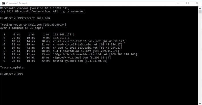
You can see the exact path of your request as well as the number of hops (left column) between the source and the destination. For each hop, there are 3 RTT values (the default of TRACERT is to send 3 data packets to test each hop).
Michael Crescimanno is a Physics professor at the Youngstown University in Ohio. The goal of the paper was to incentivize introductory students to figure out the size of the Earth rather than just accept the value on the textbook.
At the end, Michael's students were able to get to a value of Earth's radius that was within 10%-20% of today's accepted value. The precision of this measurement is comparable to Eratosthenes' original estimation using the shadows of vertical pillars in Cyrene and Alexandria in 240 BC.
Michael ended up published this paper on arXiv in 2002 with his students Snowflake Kicovic and Loren Webb.