Stochaistic: randomly determined. Even though you can see a vertical, continuous line on the graph, a step function is not continuous because its output jumps from $0$ to $1$ when crossing $z=0$ This also called a [Weighted Average](https://en.wikipedia.org/wiki/Weighted_arithmetic_mean) and though it mostly behaves like an arithmetic, regular average it has some surprising properties like [Simpson's Paradox](https://en.wikipedia.org/wiki/Simpson%27s_paradox) I think about the hyper-parameters as the parameters that are used during training but don't make it into the final trained net. This [Tensor Flow tutorial](https://www.tensorflow.org/versions/r0.11/tutorials/mnist/beginners/index.html) uses the same MNIST data set, but with a different network architecture and cost function. [Here](https://github.com/tobigithub/tensorflow-deep-learning/wiki/mnist-convolutional-example) you can find some benchmarks for that solution. Epoch: period in time. In this context, a step. In case you want to quickly freshen up your memory on logic gates: [Wikipedia - NAND Logic](https://en.wikipedia.org/wiki/NAND_logic) I understood the differences between the usage of the step-functions vs sigmoid function as the activation function of each neuron. But, I was unable to really understand the main differences of using, for example, the sigmoid function vs tanh(x) in the context of neural nets. The change of $C$, $\Delta C$, is the sum of the change in each direction $\Delta v_i$ weighted by the derivative of $C$ in that direction $\frac {\partial C}{\partial v_i}$ So, to make $C$ as small as possible, or rather $\Delta C$ a big negative number, which direction $v$ should we follow? The answer will certainly depend on $\frac{\partial C}{\partial v_i}$ The distinction between feedforward and feedback is also found in [Control Theory](https://en.wikipedia.org/wiki/Control_theory) where systems are designed to produce desired outputs from a set of changing inputs. By "calculus doesn't work" the author means that finding the closed form of the solution (exact symbolic formula) using derivatives is impractical for even the most simple networks. Even though we will not be using closed formulas, calculus is still used to derive gradient descent algorithms. In this context, the way in which the neurons are connected to each other is called the neural network's architecture. The cost functions help determine and refine the weights W, and biases B, of your neural networks. In order to do this, we use a training containing a certain number of training examples. The algorithm then ***"learns"*** by trying to minimize the difference between the data and our neural network, and while this happens it finds the best values for W and B for the entire network. One advantage comes in a "live context". As the model is operating and it gets one new data point, it can learn from it immediately without waiting for an entire batch. A disadvantage having only one data point might result in a bad estimate of $\nabla C$, which might update the model in the wrong direction, undoing some of the learning. Even though we think about the image as a 2D $28 \times 28$ vector, it is collapsed into a 1D $784$ vector. We can always collapse a matrix or tensor (a matrix that has more than 2 dimensions) into a 1D vector with as many entries as the tensor has elements. Conceptually, we can do that even if the number of rows and columns in the matrix [approach infinity](https://en.wikipedia.org/wiki/Cantor%27s_diagonal_argument)! [Cost functions](https://en.wikipedia.org/wiki/Cost_function) are used in economics, linear programming, and any field that deals with optimization. Most cost functions (including the one used in this book) are modeled after [Euclidean distance](https://en.wikipedia.org/wiki/Euclidean_distance), for which we optimize for daily. In a feedforward neural network every unit in of the layer is connected with all the units in the previous layer. These connections are not all equal: they can have different weights. Data enters at the inputs and passes flows through the network, layer by layer, until it arrives at the outputs. There is no feedback between layers, data flows continuously from one layer to the next, this is why they are called **feedforward neural networks.** The figure below shows a 2-layered network with: - an output layer with 5 units - a hidden layer with 4 units - input layer with 3 units Data enters at the bottom (input layer and flows to the top output layer)  In a binary classification (`true`, or `false`), we can also interpret the output of a sigmoid as the confidence in the result. If it outputs $0.6$ it is because it believes there is $0.6$ chance of the output being `true`. The intuition is the following: 1. We know the direction in which we want our output to change. 2. Through derivatives and approximations, we relate the change in output to the change of the parameters we control: the weights $w_k$ and biases $b_l$ 3. With that knowledge, we change the parameters in the right direction but only by a small amount, since our knowledge is only approximate and local. 4. Repeat until change is no longer possible, or you are satisfied with the net's performance. Perceptrons are not smooth, continuous functions and therefore not differentiable. Here is a video with one of my favourite explanations of gradient descent: [](https://www.youtube.com/watch?v=eikJboPQDT0) It is called an "activation function" because it determines for which values $w\cdot x + b$ will the neuron "activate": emit a non-zero output. You could imagine neurons with very strict activation functions, where only very high values of $w\cdot x+b$ activate, and lenient neurons were almost any value of $w\cdot x+b$ activates. **A training set** is a data set used to discover predictive relationships. It contains a set of examples used for learning and it helps calibrate the weights and biases of the network. We can implement a NAND gate using our `perceptron` function: ```py def nand(a, b): return perceptron([-2,-2], -3, [a, b]) ``` This is a simple example that perfectly illustrates the importance of the choice of the **weights** and the **threshold**. In this case we choose the weight $w_1$ to be predominant, so much so that the outcomes of $x_2$ and $x_3$ will not matter if $x_1$ is not accomplished. By changing the weights and the threshold we would have very different results. Here is a video of Stanford professor Andrew Ng explaining gradient descent: [](https://www.youtube.com/watch?v=eikJboPQDT0) Unlike the perceptron, the sigmoid is continuous and differentiable (traceable and smooth). This is what allows us to use derivatives to relate the change of the output $\Delta output$ to the change of the nets parameters ($\Delta w_j$ and $\Delta b$) In Python: ```py import math def sigmoid(x): return 1 / (1 + math.exp(-x)) def sigmoid_neuron(weights, bias, inputs): return sigmoid(-dot(weights,inputs) - bias) ``` Here is a video of Stanford professor Andrew Ng explaining what a cost function is and how it helps fit data: [](https://www.youtube.com/watch?v=qM4EBJ_dbVI) Though useful, the comparison between function abstraction in programming languages and abstraction by neural network layers breaks when it comes to debugging. The lower levels of a program were also written by humans and we can understand them (i.e. `replace-substring` consists of `find-substring`, `remove-substring`, and `concat-string`). The lower levels of a neural network are a set of real numbers that the algorithm discovered and don't necessarily have relationships to concepts we can understand. The perceptron is an extreme case of a sigmoid neutron when the absolute value of $z$: $$ z \equiv w\cdot x + b$$ is either very large of very small. Using the new notation where we introduce the bias, b: $$b = - \text{threshold.}$$ The likelihood of the perceptron firing (returning 1) increases as the bias increases. We can easily rewrite our basic perceptron Python program taking the bias into account: ```python from numpy import dot def perceptron(weights, bias, inputs): if dot(weights, inputs) + bias <= 0: return 0 else: return 1 ``` An **artificial neuron** is a mathematical function that mimics biological neurons. Artificial neurons are the constitutive units in artificial neural networks. To learn more visit: - [Wikipedia - Artificial neuron](https://en.wikipedia.org/wiki/Artificial_neuron) - [Wikipedia - Perceptron](https://en.wikipedia.org/wiki/Perceptron) By "artificial neuron" he means the basic unit of computation upon which the learning algorithms are based. Those units resemble models of actual neurons. A perceptron is a computational model of a single neuron and it is the simplest neural network possible. A perceptron consists of one or more inputs, a processor, **and a single output**. It follow a feed-forward”model: 1. inputs are sent into the neuron, 2. they are processed, and 3. they result in an output. Alternatively we can use the [dot product](https://en.wikipedia.org/wiki/Dot_product) to think about the weights and the inputs as vectors: \[ output = \vec{w} \cdot \vec{x} \le threshold \] which can be implemented with the very concise Python progam: ```python from numpy import dot def perceptron(weights, threshold, inputs): if dot(weights, inputs) <= threshold: return 0 else: return 1 ``` Instead of exactly defining what a handwritten ***9*** is, and think about the all the potential edge cases, we simply show the machine a lot of different ***9*** 's and let it ***learn and come up with rules*** for what a ***9*** is. The heuristic techniques of neural net designs include such ideas as varying the learning rate, using momentum and rescaling variables. You can learn more about these heuristics here: - [Momentum and Learning Rate Adaptation](http://www.willamette.edu/~gorr/classes/cs449/momrate.html) - [An overview of gradient descent optimization algorithms](http://sebastianruder.com/optimizing-gradient-descent/) NAND gates and NOR gates are called Universal Gates because you can build any boolean circuit using them. In the [Wikipedia page for NAND's](https://en.wikipedia.org/wiki/NAND_logic) you can see all the basic gates like AND and OR implemented in terms of NANDs. As an example, here is the implementation of Q=XOR(A,B):  The value of $\eta$ is important: - if $\eta$ is too small gradient descent will take too long to reach the global minimum - if $\eta$ is too large gradient descent can overshoot the global minimum and converge to a local minimum instead A good value of $\eta$ is thus important in order to converge to the global minimum and to do so quickly. This video discusses the differences in $\eta$ ($\alpha$ in the video) and how it impacts gradient descent. [](https://youtu.be/Fn8qXpIcdnI?list=PLLH73N9cB21V_O2JqILVX557BST2cqJw4&t=341) If one dimension, we can think about it as a cart moving through a rollercoaster:  We want to get to the lowest point in the ride. At any given point, we can move the cart left or right depending on the slope at that point. If the cart starts at $W$, we'll always move right until $X$, the _global minimum_. If we start to the left of $Y$ we'll also end in $X$. But if we start right of $Y$, we'll end in $Z$ which even thought is a _local minimum_ (once you are there you don't see how to continue going down) it is not the _global minimum_. Missing the global minimum for a local minimum is one of the risks of the hill climbing algorithm. This is a linear approximation that is only valid around one point. If you calculate $\nabla C_a$ for a point $x_a$, you can't use that same $\nabla C_a$ for an another $x_b$ that is far away from $x_a$ @Gustavo $\tanh$ would be a better choice than the sigmoid. I believe the author just the sigmoid for simplicity reasons: \begin{eqnarray*} \newcommand{\exp}{\mathrm{e}^} \sigma(x) = \frac{1}{(1+\exp{-x})} \end{eqnarray*} and: \begin{eqnarray*} \newcommand{\exp}{\mathrm{e}^} \tanh(x) = \frac{\exp{x} - \exp{-x}}{\exp{x} + \exp{-x}} = 2\sigma(2x) - 1 \end{eqnarray*} Later in [chapter 6. of the book](http://fermatslibrary.com/s/deep-learning#email-newsletter) he will do some experiments with the $\tanh$. If you want to learn more about the reasons why one activation function is better that the other read [Efficient Backprop by Le Cunn et al.](http://yann.lecun.com/exdb/publis/pdf/lecun-98b.pdf) (section 4.4). [Pierre François Verhulst](https://en.wikipedia.org/wiki/Pierre_Fran%C3%A7ois_Verhulst) encountered the sigmoid function when studying how do populations change when living in an environment with limited resources. The Sigmoid is an activation function of the neural network. Some of its properties are: - Real valued and differentiable - Analytic tractability for the differentiation operation - The output shows if the neuron is firing or not The figure below shows different examples of *smooth* sigmoid functions (all functions are normalized in such a way that their slope at the origin is 1). Other interesting resources about the sigmoid and other activations functions: - [Wolfram - Sigmoid Function](http://mathworld.wolfram.com/SigmoidFunction.html) - [Other types of activation functions](https://en.wikipedia.org/wiki/Activation_function)  This is the first chapter of Michael Nielsen's book **Neural Networks and Deep Learning**. Michael Nielsen in his own words: ***"I'm a scientist, writer, and programmer."*** He is a Quantum Physicist by training, specializing in the fields of Quantum Information and Quantum Computation. As of 2015 he has been working as a Research Fellow at Y Combinator Research. This book is one of the best introductions to Machine Learning. The first chapter focuses on the recognition of handwritten digits. You will find added content, like links to videos and solutions to the exercises proposed by the author. More resources: - [Michael Nielsen's website](http://michaelnielsen.org) - [Neural Networks and Deep Learning](http://neuralnetworksanddeeplearning.com/index.html) - [Github: Neural Networks and Deep Learning](https://github.com/mnielsen/neural-networks-and-deep-learning) The batches are randomized for the same reason arrays are shuffled before using the [Quicksort sorting algorithm](https://en.wikipedia.org/wiki/Quicksort): even though the strategy we are using is optimal for most cases, it is disastrous for a set of expected cases. Imagine if the inputs were organized so that all $0$ images came together, then $1$s and so on. Each mini batch wouldn't contain the information to make the net a better digit classifier, but rather to find only one of the digits. Each batch would over step in one direction, and part of that work would have to be reversed by the next batch. Randomizing the batches makes this very unlikely. Nielsen strikes the perfect balance between the mechanics of neural networks while providing high-level intuition on their capabilities and limitations. Unlike most of the Machine Learning literature, it assumes only basic math and basic programming. If you are curious on what is behind all the recent hype , this book is the perfect way to start. Functions for which a small change in input causes a bounded change in its output are called [differentiable](https://en.wikipedia.org/wiki/Differentiable_function). We can describe them as smooth, since their curves have no sharp turns. For a function to be differentiable, it also needs to be [continuous](https://en.wikipedia.org/wiki/Continuous_function): there should be no abrupt jumps in the output. We can describe them as traceable: as you trace the curve with your pencil, you shouldn't need to lift it to continue. 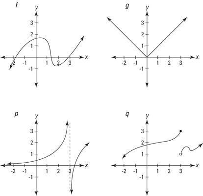These concepts are easier to see in a diagram:  * $f$ is both continuous and differentiable (traceable and smooth overall) * $g$ is continuous in all points but non differentiable in $x=0$ (traceable but not smooth) * $p$ and $q$ are continuous and differentiable in all points but $x=3$ Perceptrons use learning algorithms to automatically tune the weights and biases of the network. A learning algorithm is an adaptive method by which a network of perceptrons auto-tines itself to implement the desired behavior. This is accomplished by providing examples of the desired input-output mapping to the network. A correction step is executed iteratively until the network learns to produce the desired response, see diagram below.  The figure below shows an example of an image with 9 pixels, each pixel is an input neuron for the neural network. The output layer contains one single neuron with output value V, where V is either greater or less than 0.5.  Let's start by showing that the formula for any given perceptron doesn't change when multiplying by a constant. If none of the perceptrons change, it follows that the network doesn't change either. We start with the formula for a perceptron: \[ \vec{w} \cdot \vec{x} + b \le 0 \] we multiply both the weights $\vec{w}$ and the bias $b$ by $c$: \[c\vec{w} \cdot \vec{x} + c b \le 0\] (the inequality is unchaged because $c \gt 0$). We extract the common $c$ from the difference: \[c (\vec{w} \cdot \vec{x} + b) \le 0\] If $c>0$, the only way in which the composite term $c(\vec{w}\cdot\vec{x}+b)$ is negative is if the second term is negative. That is: \[ \vec{w} \cdot \vec{x} + b \le 0 \] which demonstrates that the boolean function we are calculating remains unchanged. Lets first remember what happens to $\sigma(z)$ when its input grows to $\infty$: \[ \lim_{z\to\infty} \sigma(z) = 1 \] \[ \lim_{z\to-\infty} \sigma(z) = 0 \] From those two limits we can see that $\sigma(z)$ behaves like a perceptron (only outputs $1$ or $0$) if its inputs are constraint to either $-\infty$ or $\infty$. A sigmoid neuron is one where the output is given by: \[ \sigma(\vec{w} \cdot \vec{x} + b) \] What happens if we multiply $\vec{w}$ and $b$ by $c\to\infty$: \[\lim_{c\to\infty}\sigma(c(\vec{w}\cdot\vec{x} + b))\] If $\vec{w}\cdot\vec{x} + b > 0$ we get: \[\lim_{c\to\infty}\sigma(\infty)=1\] If $\vec{w}\cdot\vec{x} + b < 0$ we get: \[\lim_{c\to\infty}\sigma(-\infty)=0\] If $\vec{w}\cdot\vec{x} + b = 0$ we get: \[\lim_{c\to\infty}\sigma(0)=\frac{1}{2}\] Therefore we see that multiplying $\vec{w}$ and $b$ by a very big constant transforms a sigmoid neuron into a perceptron _as long as the input does not result in_ $\vec{w}\cdot\vec{x}+b=0$ Notice that $\sigma(z)$ approaches $1$ as $z$ grows towards $\infty$ and approaches $0$ as $z$ approaches $-\infty$. We can write that as: \[\lim_{z\to\infty} \sigma(z) = \lim_{z\to\infty}\frac{1}{1+e^{-z}}=1 \] \[\lim_{z\to-\infty} \sigma(z) = \lim_{z\to-\infty}\frac{1}{1+e^{-z}}=0 \] **The Input Layer:** A neural network has exactly one input layer The number of neurons comprising this layer is completely and uniquely determined once you know the shape of your training data. **The Output layer:** Like the Input layer, every neural network has exactly one output layer. The size of the output layer is determined by the chosen model configuration. **The Hidden Layers:** There is a performance difference from adding additional hidden layers. One hidden layer is sufficient for the large majority of problems. For most problems, one could set the hidden layer configuration using just two rules: - number of hidden layers equals one - the number of neurons in that layer is the mean of the neurons in the input and output layers. You can read more about this topic here: [How to choose the number of hidden layers and nodes in a feedforward neural network?](http://stats.stackexchange.com/questions/181/how-to-choose-the-number-of-hidden-layers-and-nodes-in-a-feedforward-neural-netw) Let's start thinking about what we want to find: the weights $w_{ij}$ and biases $b_j$ that take an input $\vec{x} \in \mathbb{R}^{10} $ from the old output layer and transform it into $\vec{y} \in \mathbb{R}^4$, the new binary output layer. If we are using perceptrons, each individual output looks like: \[ y_j = w_{ij}x_i + b_j \le 0 \] where $x_i = 1$ if $i$ is the recognized character and $0$ otherwise. Those 4 equations ($\vec{y}$ has 4 components) can be rewritten in matrix form: \[\vec{y} = W\vec{x} + \vec{b}\] where $W\in\mathbb{R}^{4x10}$ and $\vec{b}\in\mathbb{R}^4$. Now to the question: how do we transform a number from $0$ to $9$ encoded in a vector of length $10$ with many $0$s and a $1$ in the desired place into a binary vector of length $4$? \[\vec{x} =[0,0,0,1,0,0,0,0,0,0,0]^T = 3\] \[\vec{y} =[1,0,1,0,0]^T = 3 \] If we assume that $\vec{x}$ will be $1$ only in one row, we can create a matrix $W$ where each column $i$ is the binary encoding of the number $i$. Then when we multiply $W\vec{x}$ only the $i_{th}$ column will survive, giving us the desired binary number: \[\vec{y} = W\vec{x}\] \[\vec{y} = \begin{bmatrix} 0&1&0&1&0&1&0&1&0&1\\ 0&0&1&1&0&0&1&1&0&0\\ 0&0&0&0&1&1&1&1&0&0\\ 0&0&0&0&0&0&0&0&1&1 \end{bmatrix} \vec{x} \] Notice how the $0_{th}$ column is $0$ in binary, the first column is $1$ in binary, and so on. But what happens if the input has $0.99$ and $0.01$? Each column gets some extra $0.01$: * If the column should be $1$, it is actually $0.99+3\cdot0.01=1.02$ * If the column should be $0$, it is actually $4\cdot0.01=0.04$ To discern the signal from the noise, we can add biases $b_j \in (-1.02,-0.04)$, for example $b_j = -0.5$. Now: * If the column should be $1$, it is $0.99+3\cdot0.01- 0.5=0.52 > 0$ * If the column should be $0$, it is actually $4\cdot0.01-0.5 =-0.46 < 0$ Our goal is to pick in which direction we are going to step, $\Delta v$, so that we go as downwards as possible; the length of the step, $|\Delta C|$, should be as big as possible. We know they relate through $\nabla C$: \[\Delta C \approx \nabla C \cdot \Delta v \] \[\Delta C^2 \approx (\nabla C \cdot \Delta v)^2 \] \[ \Delta C^2 \approx (\nabla C \cdot \Delta v) (\nabla C \cdot \Delta v) \] From the Cauchy-Schwarz inequality we know that the square of the dot product of two vectors is bounded: \[ \Delta C^2 = (\nabla C \cdot \Delta v)^2 \le (\nabla C \cdot \nabla C)(\Delta v \cdot \Delta v) \] The intuition behind this inequality is the following: the dot product of two vectors calculates how well does one vector "project" into the other. 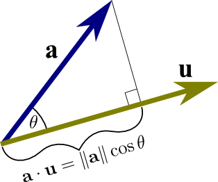If you draw two vectors $a$ and $u$:  their dot product calculates the length of $a$ once you try to fit it/project it into $u$. If the vectors are parallel, then the projection is as long as it can be. If they are perpendicular, the projection is $0$. Since we want $|\Delta C|$ to be as big as possible, we should pick the $\Delta v$ that gets us to the bound: \[ (\nabla C \cdot \Delta v) (\nabla C \cdot \Delta v) = (\nabla C \cdot \nabla C) (\Delta v \cdot \Delta v) \] and since it is a dot product, we should make both $\Delta v$ parallel to $\nabla C$: \[\Delta v = \eta \nabla C\] where $\eta$ is a constant that relates their lengths (but keeps the vectors parallel). But we are not done, we have another constraint: $|| \Delta v || = \epsilon $ So we pick $\eta$ to fit it: \[ ||\Delta v|| = \epsilon = |\eta| \cdot ||\nabla C|| \] \[ |\eta| = \frac{\epsilon}{||\nabla C||} \] So then finally: \[\Delta v = \frac{-\epsilon \nabla C}{||\nabla C||} \]